It may happen that we created an index and yet PostgreSQL doesn’t use it. What could be the reason and how to fix it? We identified 11 distinct scenarios. Read on to find out.
Important Things
Indexes may be tricky. We already covered how they work in another article. Let’s quickly recap important parts about how they work.
How Indexes Work
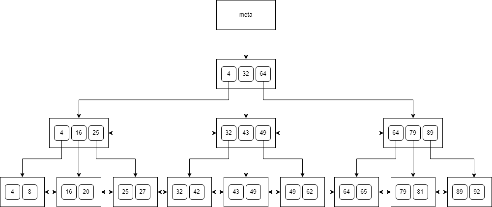
The B-tree is a self-balancing tree data structure that maintains a sorted order of entries, allowing for efficient searches, insertions, and deletions in logarithmic time—unlike regular heap tables, which operate in linear time. B-trees are an extension of binary search trees, with the key distinction that they can have more than two children. B-trees in PostgreSQL satisfy the following:
- Every node has at most 3 children.
- Every node (except for the root and leaves) has at least 2 children.
- The root node has at least two children (unless the root is a leaf).
- Leaves are on the same level.
- Nodes on the same level have links to siblings.
- Each key in the leaf points to a particular TID.
- Page number 0 of the index holds metadata and points to the tree root.
We can see a sample B-tree below:
When inserting a key into a full node, the node must be split into two smaller nodes, with the key being moved up to the parent. This process may trigger further splits at the parent level, causing the change to propagate up the tree. Likewise, during key deletion, the tree remains balanced by merging nodes or redistributing keys among sibling nodes.
For searching, we can apply the binary search algorithm. Suppose we're searching for a value that appears in the tree only once. Here's how we would navigate the tree while looking for 62:
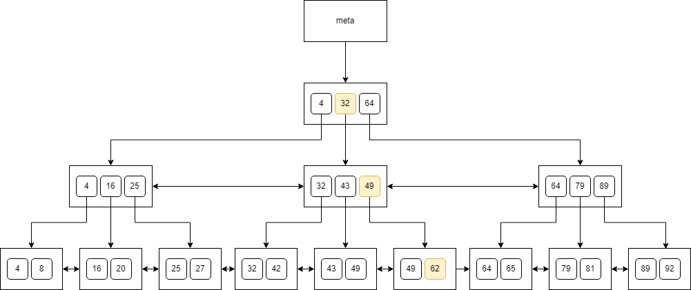
You can see that we just traverse the nodes top-down, check the keys, and finally land at a value. A similar algorithm would work for a value that doesn’t exist in the tree.
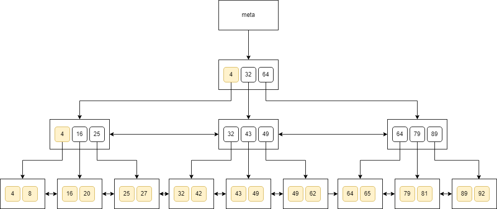
This is more obvious when we look for all the values that are greater than 0:
How Database Estimates The Cost
The index cost consists of the start-up cost and the run cost.
The start-up cost depends on the number of tuples in the index and the height of the index. It is specified as cpu_operator_cost multiplied by the ceiling of the base-2 logarithm of the number of tuples plus the height of the tree multiplied by 50.
The run cost is the sum of the CPU cost (for both the table and the index) and the I/O cost (again, for the table and the index).
The CPU cost for the index is calculated as the sum of constants cpu_index_tuple_cost and qual_op_cost (which are 0.005 and 0.0025 respectively) multiplied by the number of tuples in the index multiplied by the selectivity of the index.
Selectivity of the index is the estimate of how many values inside the index would match the filtering criteria. It is calculated based on the histogram that captures the counts of the values. The idea is to divide the column’s values into groups of approximately equal populations to build the histogram. Once we have such a histogram, we can easily specify how many values should match the filter.
The CPU cost for the table is calculated as the cpu_tuple_cost (constant 0.01) multiplied by the number of tuples in the table multiplied by the selectivity. Notice that this assumes that we’ll need to access each tuple from the table even if the index is covering.
The I/O cost for the index is calculated as the number of pages in the index multiplied by the selectivity multiplied by the random_page_cost which is set to 4.0 by default.
Finally, the I/O cost for the table is calculated as the sum of the number of pages multiplied by the random_page_cost and the index correlation multiplied by the difference between the worst-case I/O cost and the best-case I/O cost. The correlation indicates how much the order of tuples in the index is aligned with the order of tuples in the table. It can be between -1.0 and 1.0.
All these calculations show that index operations can be beneficial if we extract only a subset of rows. It’s no surprise that the index scans will be even more expensive than the sequential scans, but the index seeks will be much faster.
Index Construction
Indexes can be built on multiple columns. The order of columns matters, the same as the order of values in the column (whether it’s ascending or descending).
The index requires a way to sort values. The B-tree index has an inherent capability of value organization within certain data types, a feature we can exploit quite readily for primary keys or GUIDs as the order is typically immutable and predictable in terms of such scenarios due to their 'built-in' nature which aligns with increasing values. However, when dealing with complex custom datatypes - say an object containing multiple attributes of varying data types – it’s not always apparent how these might be ordered within a B-tree index given that they do not have an inherent ordering characteristic, unlike primitive (basic) or standardized composite data types such as integers and structured arrays.
Consequently, for situations where we deal with complex datatypes - consider the two-dimensional points in space that lack any natural order due to their multi-attribute nature – one might find it necessary to incorporate additional components within our indexing strategy or employ alternative methods like creating multiple indexes that cater specifically towards different sorting scenarios. PostgreSQL provides a solution for this through operator families, wherein we can define the desired ordering characteristics of an attribute (or set of attributes) in complex datatypes such as two-dimensional points on Cartesian coordinates when considering order by X or Y values separately – essentially providing us with customizable flexibility to establish our unique data arrangement within a B-tree index.
How to Check If My Index Is Used
We can always check if the index was used with EXPLAIN ANALYZE. We use it like this:
EXPLAIN ANALYZE
SELECT …
This query returns a textual representation of the plan with all the operations listed. If we see the index scan among them, then the index has been used.
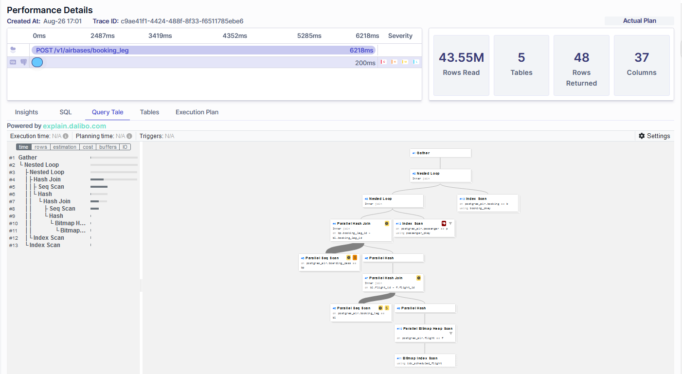
Also, Metis shows which indexes were used:
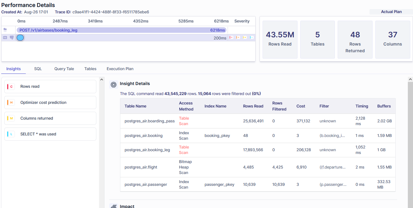
Metis also shows query visualization:
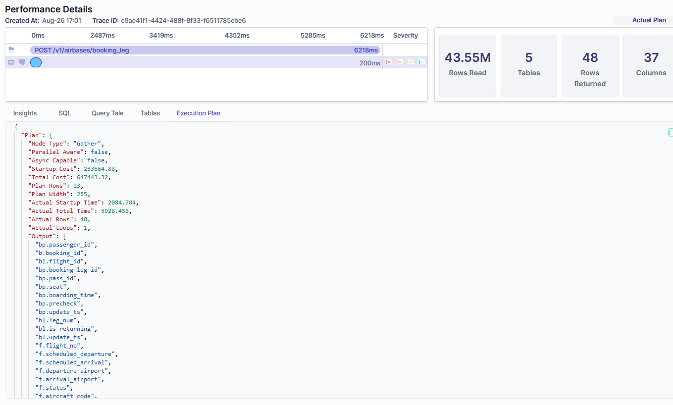
Metis also captures an execution plan so you can analyze it with other tools if needed:
Why Isn’t My Index Used
Let’s now go through the reasons why an index may not be used. Even though we focus on B-tree indexes here, similar issues can apply to other index types (BRIN, GiST, GIN, etc.).
The general principle is: that either the database can’t use the index, or the database thinks that the index will make the query slower. All the scenarios we explain below simply come down to these two principles and only manifest themselves differently.
The Index Will Make The Query Slower
Let’s start with the cases when the database thinks the index will make the query slower.
Table Scan Is Cheaper
The very first reason is that the table scan may be faster than the index. This can be the case for small tables.
A trivial example includes the following. Let’s create a table:
CREATE TABLE people (id INT, name VARCHAR, last_name VARCHAR);
Let’s insert two rows:
INSERT INTO people VALUES (1, 'John', 'Doe'), (2, 'Mary', 'Alice')
Let’s now create an index:
CREATE INDEX people_idx ON people(id);
If we now try to query the table and get the execution plan, we get the following:
EXPLAIN ANALYZE
SELECT *
FROM people
WHERE id = 2
Seq Scan on people  (cost=0.00..1.02 rows=1 width=36) (actual time=0.014..0.016 rows=1 loops=1)
  Filter: (id = 2)
  Rows Removed by Filter: 1
Planning Time: 0.068 ms
Execution Time: 0.123 ms
We can see the database decided to scan the table instead of using an index. That is because it was cheaper to scan the table. We can disable scans if possible with:
set enable_seqscan=off
Let’s now try the query:
EXPLAIN ANALYZE
SELECT *
FROM people
WHERE id = 2
Index Scan using people_idx on people (cost=0.13..8.14 rows=1 width=68) (actual time=0.064..0.066 rows=1 loops=1)
Index Cond: (id = 2)
Planning Time: 0.066 ms
Execution Time: 0.170 ms
We can see that the sequential scan cost was 1.02 whereas the index scan cost was 8.14. Therefore, the database was right to scan the table.
The Query Is Not Selective Enough
Another reason is that the query may not be selective enough. This is the same case as before, only it manifests itself differently. This time, we don’t deal with small tables, but we extract too many rows from the table.
Let’s add more rows to the table:
INSERT INTO people (
    	WITH RECURSIVE numbers(n) AS (
            	VALUES (3)
            	UNION ALL
            	SELECT n+1 FROM numbers WHERE n < 1000
    	)
    	SELECT n, 'Jack ' || n, 'Dean' FROM numbers
)
Let’s now query like this:
EXPLAIN ANALYZE
SELECT *
FROM people
WHERE id <= 999
Seq Scan on people  (cost=0.00..7.17 rows=5 width=68) (actual time=0.011..0.149 rows=999 loops=1)
  Filter: (id <= 999)
  Rows Removed by Filter: 1
Planning Time: 0.072 ms
Execution Time: 0.347 ms
We can see the sequential scan again. Let’s see the cost when we disable scans:
Index Scan using people_idx on people  (cost=0.28..47.76 rows=999 width=17) (actual time=0.012..0.170 rows=999 loops=1)
  Index Cond: (id <= 999)
Planning Time: 0.220 ms
Execution Time: 0.328 ms
So we can see the scan is 7.17 versus 47.76 for the index scan. This is because the query extracts nearly all the rows from the table. It’s not very selective. However, if we try to pick just one row, we should get this:
EXPLAIN ANALYZE
SELECT *
FROM people
WHERE id = 2
Index Scan using people_idx on people  (cost=0.28..8.29 rows=1 width=17) (actual time=0.018..0.020 rows=1 loops=1)
  Index Cond: (id = 2)
Planning Time: 0.064 ms
Execution Time: 0.126 ms
Keep in mind that partial indexes may be less or more selective and affect the execution plans.
LIMIT Clause Misleads The Database
The LIMIT clause may mislead the database and make it think that the sequential scan will be faster.
Let’s take this query:
EXPLAIN ANALYZE
SELECT *
FROM people
WHERE id <= 50
LIMIT 1
We want to find the rows with id less or equal to fifty. However, we take only one row. The plan looks like this:
Limit  (cost=0.00..0.39 rows=1 width=17) (actual time=0.016..0.017 rows=1 loops=1)
  ->  Seq Scan on people  (cost=0.00..19.50 rows=50 width=17) (actual time=0.015..0.015 rows=1 loops=1)
    	Filter: (id <= 50)
Planning Time: 0.073 ms
Execution Time: 0.131 ms
We can see the database decided to scan the table. However, let’s change the LIMIT to three rows:
EXPLAIN ANALYZE
SELECT *
FROM people
WHERE id <= 50
LIMIT 3
Limit  (cost=0.28..0.81 rows=3 width=17) (actual time=0.018..0.019 rows=3 loops=1)
  ->  Index Scan using people_idx on people  (cost=0.28..9.15 rows=50 width=17) (actual time=0.017..0.018 rows=3 loops=1)
    	Index Cond: (id <= 50)
Planning Time: 0.073 ms
Execution Time: 0.179 ms
This time we get the index scan. This clearly shows that the LIMIT clause affects the execution plan. However, notice that both of the queries executed in 131 and 179 milliseconds respectively. If we disable the scans, we get the following:
Limit  (cost=0.28..0.81 rows=3 width=17) (actual time=0.019..0.021 rows=3 loops=1)
  ->  Index Scan using people_idx on people  (cost=0.28..9.15 rows=50 width=17) (actual time=0.018..0.019 rows=3 loops=1)
    	Index Cond: (id <= 50)
Planning Time: 0.074 ms
Execution Time: 0.090 m
In this case, the table scan was indeed faster than the index scan. This obviously depends on the query we execute. Be careful with using LIMIT.
Inaccurate Statistics Mislead The Database
As we saw before, the database uses many heuristics to calculate the query cost. The query planner estimates are based on the number of rows that each operation will return. This is based on the table statistics that may be off if we change the table contents significantly or when columns are dependent on each other (with multivariate statistics).
As explained in the PostgreSQL documentation, statistics like reltuples and relpages are not updated on the fly. They get updated periodically or when we run commands like VACUUM, ANALYZE, or CREATE INDEX.
Always keep your statistics up to date. Run ANALYZE periodically to make sure that your numbers are not off, and always run ANALYZE after batch-loading multiple rows. You can also read more in PostgreSQL documentation about multivariate statistics and how they affect the planner.
The Database Is Configured Incorrectly
The planner uses various constants to estimate the query cost. These constants should reflect the hardware we use and the infrastructure backing our database.
One of the prominent examples is random_page_cost. This constant is meant to represent the cost of accessing a data page randomly. It’s set to 4 by default whereas the seq_page_cost constant is set to 1. This makes a lot of sense for HDDs that are much slower for random access than the sequential scan.
However, SSDs and NVMes do not suffer that much with random access. Therefore, we may want to change this constant to a much lower value (like 2 or even 1.1). This heavily depends on your hardware and infrastructure, so do not tweak these values blindly.
There Are Better Indexes
Another case for not using our index is when there is a better index in place.
Let’s create the following index:
CREATE INDEX people_idx2 ON people(id) INCLUDE (name);
Let’s now run this query:
EXPLAIN ANALYZE
SELECT id, name
FROM people
WHERE id = 123
Index Only Scan using people_idx2 on people  (cost=0.28..8.29 rows=1 width=12) (actual time=0.026..0.027 rows=1 loops=1)
  Index Cond: (id = 123)
  Heap Fetches: 1
Planning Time: 0.208 ms
Execution Time: 0.131 ms
We can see it uses people_idx2 instead of people_idx. The database could use people_idx as well but people_idx2 covers all the columns and so can be used as well. We can drop people_idx2 to see how it affects the query:
Index Scan using people_idx on people  (cost=0.28..8.29 rows=1 width=12) (actual time=0.010..0.011 rows=1 loops=1)
  Index Cond: (id = 123)
Planning Time: 0.108 ms
Execution Time: 0.123 ms
We can see that using people_idx had the same estimated cost but was faster. Therefore, always tune your indexes to match your production queries.
The Index Can’t Be Used
Let’s now examine cases when the index can’t be used for some technical reasons.
The Index Uses Different Sorting
Each index must keep the specific order of rows to be able to run the binary search. If we query for rows in a different order, we may not be able to use the index (or we would need to sort all the rows afterward). Let’s see that.
Let’s drop all the indexes and create this one:
CREATE INDEX people_idx3 ON people(id, name, last_name)
Notice that the index covers all the columns in the table and stores them in ascending order for every column. Let’s now run this query:
EXPLAIN ANALYZE
SELECT id, name
FROM people
ORDER BY id, name, last_name
Index Only Scan using people_idx3 on people  (cost=0.15..56.90 rows=850 width=68) (actual time=0.006..0.007 rows=0 loops=1)
  Heap Fetches: 0
Planning Time: 0.075 ms
Execution Time: 0.117 ms
We can see we used the index to scan the table. However, let’s now sort the name DESC:
EXPLAIN ANALYZE
SELECT id, name
FROM people
ORDER BY id, name DESC, last_name
Sort  (cost=66.83..69.33 rows=1000 width=17) (actual time=0.160..0.211 rows=1000 loops=1)
  Sort Key: id, name DESC, last_name
  Sort Method: quicksort  Memory: 87kB
  ->  Seq Scan on people  (cost=0.00..17.00 rows=1000 width=17) (actual time=0.009..0.084 rows=1000 loops=1)
Planning Time: 0.120 ms
Execution Time: 0.427 ms
We can see the index wasn’t used. That is because the index stores the rows in a different order than the query requested. Always configure indexes accordingly to your queries to avoid mismatches like this one.
The Index Stores Different Columns
Another example is when the order matches but we don’t query the columns accordingly. Let’s run this query:
EXPLAIN ANALYZE
SELECT id, name
FROM people
ORDER BY id, last_name
Sort  (cost=66.83..69.33 rows=1000 width=17) (actual time=0.157..0.198 rows=1000 loops=1)
  Sort Key: id, last_name
  Sort Method: quicksort  Memory: 87kB
  ->  Seq Scan on people  (cost=0.00..17.00 rows=1000 width=17) (actual time=0.012..0.086 rows=1000 loops=1)
Planning Time: 0.081 ms
Execution Time: 0.388 ms
Notice that the index wasn’t used. That is because the index stores all three columns but we query only two of them. Again, always tune your indexes to store the data you need.
The Query Uses Functions Differently
Let’s now run this query with a function:
EXPLAIN ANALYZE
SELECT id, name
FROM people
WHERE abs(id) = 123
Seq Scan on people  (cost=0.00..22.00 rows=5 width=12) (actual time=0.019..0.087 rows=1 loops=1)
  Filter: (abs(id) = 123)
  Rows Removed by Filter: 999
Planning Time: 0.124 ms
Execution Time: 0.181 ms
We can see the index wasn’t used. That is because the index was created on a raw value of the id column, but the query tries to get abs(id). The engine could do some more extensive analysis to understand that the function doesn’t change anything in this case, but it decided not to.
To make the query faster, we can either not use the function in the query (recommended) or create an index for this query specifically:
CREATE INDEX people_idx4 ON people(abs(id))
And then we get:
Bitmap Heap Scan on people  (cost=4.31..11.32 rows=5 width=12) (actual time=0.022..0.024 rows=1 loops=1)
  Recheck Cond: (abs(id) = 123)
  Heap Blocks: exact=1
  ->  Bitmap Index Scan on people_idx4  (cost=0.00..4.31 rows=5 width=0) (actual time=0.016..0.017 rows=1 loops=1)
    	Index Cond: (abs(id) = 123)
Planning Time: 0.209 ms
Execution Time: 0.159 ms
The Query Uses Different Data Types
Yet another example is when we store values with a different data type in the index. Let’s run this query:
EXPLAIN ANALYZE
SELECT id, name
FROM people
WHERE id = 123::numeric
Seq Scan on people  (cost=0.00..22.00 rows=5 width=12) (actual time=0.030..0.156 rows=1 loops=1)
  Filter: ((id)::numeric = '123'::numeric)
  Rows Removed by Filter: 999
Planning Time: 0.093 ms
Execution Time: 0.278 ms
Even though 123 and 123::numeric represent the same value, we can’t use the index because it stores integers instead of numeric types. To fix the issue, we can create a new index targeting this query or change the casting to match the data type:
EXPLAIN ANALYZE
SELECT id, name
FROM people
WHERE id = 123::int
Bitmap Heap Scan on people  (cost=4.18..12.64 rows=4 width=36) (actual time=0.005..0.006 rows=0 loops=1)
  Recheck Cond: (id = 123)
  ->  Bitmap Index Scan on people_idx3  (cost=0.00..4.18 rows=4 width=0) (actual time=0.004..0.004 rows=0 loops=1)
    	Index Cond: (id = 123)
Planning Time: 0.078 ms
Execution Time: 0.088 ms
Operators Are Not Supported
Yet another example of when an index can’t be used is when we query data with an unsupported operator. Let’s create such an index:
CREATE INDEX people_idx5 ON people(name)
Let’s now query the table with the following;
EXPLAIN ANALYZE
SELECT name
FROM people
WHERE name = 'Jack 123'
Index Only Scan using people_idx5 on people  (cost=0.28..8.29 rows=1 width=8) (actual time=0.025..0.026 rows=1 loops=1)
  Index Cond: (name = 'Jack 123'::text)
  Heap Fetches: 1
Planning Time: 0.078 ms
Execution Time: 0.139 ms
We can see the index worked. However, let’s now change the operator to ILIKE:
EXPLAIN ANALYZE
SELECT name
FROM people
WHERE name ILIKE 'Jack 123'
Seq Scan on people  (cost=0.00..19.50 rows=1 width=8) (actual time=0.075..0.610 rows=1 loops=1)
  Filter: ((name)::text ~~* 'Jack 123'::text)
  Rows Removed by Filter: 999
Planning Time: 0.130 ms
Execution Time: 0.725 ms
We can see the database decided not to use an index. This is because we use the ILIKE operator which is not supported with a regular B-tree index. Therefore, always use the appropriate operators to use indexes efficiently.
Keep in mind that operators can be prone to various settings. For instance different collation may cause an index to be ignored.
Testing Indexes With HypoPG
To test various indexes, we don’t need to create them. We can use HypoPG extension that can analyze the index without creating it in the database.
Let’s see that in action. Drop all the indexes and run the following query:
EXPLAIN ANALYZE
SELECT *
FROM people
WHERE id = 2
Seq Scan on people  (cost=0.00..19.50 rows=1 width=17) (actual time=0.011..0.079 rows=1 loops=1)
  Filter: (id = 2)
  Rows Removed by Filter: 999
Planning Time: 0.103 ms
Execution Time: 0.163 ms
We can see, that no index was used as there were no indexes at all. We can now see what would happen if we had an index. Let’s first pretend as we created it:
SELECT *
FROM hypopg_create_index('CREATE INDEX ON people (id)');
13563 <13563>btree_people_id
And let’s now ask the database if it would be used (notice there is no ANALYZE):
EXPLAIN
SELECT *
FROM people
WHERE id = 2
Index Scan using "<13563>btree_people_id" on people (cost=0.00..8.01 rows=1 width=17)
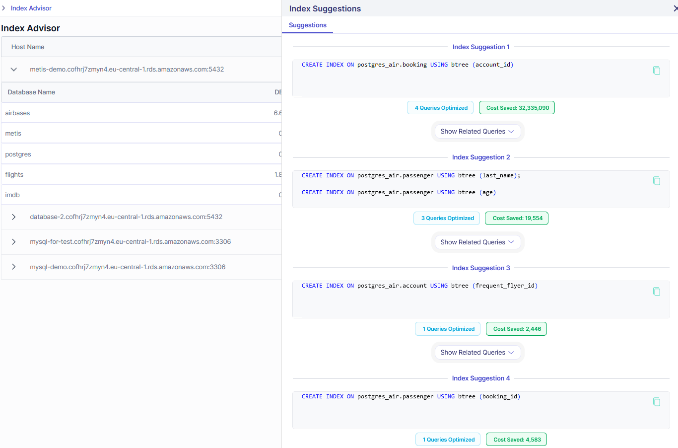
This way we can test various indexes. This is also what Metis does behind the scenes with its Index Advisor:
Summary
Indexes may be tricky and there are many reasons why they are not used. However, ultimately it all goes down to either the database not being able to use the index or thinking that it would make things slower. Fortunately, we can easily verify if indexes are used with EXPLAIN ANALYZE, and we can also test new indexes with HypoPG. Metis does all of that automatically, so you don’t need to do the hard work anymore. Use Metis and put your indexes on steroids.