PostgreSQL Everywhere and For Everything

PostgreSQL is one of the most popular SQL databases. It’s a go-to database for many projects dealing with Online Transaction Processing systems. However, PostgreSQL is much more versatile and can successfully handle less popular SQL scenarios and workflows that don’t use SQL at all. In this blog post, we’ll see other scenarios where PostgreSQL shines and will explain how to use it in these cases.

How It All Started

Historically, we focused on two distinct database workflows: Online Transaction Processing (OLTP) and Online Analytical Processing (OLAP).

OLTP represents the day-to-day applications that we use to create, read, update, and delete (CRUD) data. Transactions are short and touch only a subset of the entities at once, and we want to perform all these transactions concurrently and in parallel. We aim for the lowest latency and the highest throughput as we need to execute thousands of transactions each second.

OLAP focuses on analytical processing. Typically after the end of the day, we want to recalculate many aggregates representing our business data. We summarize the cash flow, recalculate users’ preferences, or prepare reports. Similarly, after each month, quarter, or year, we need to build business performance summaries and visualize them with dashboards. Those workflows are completely different from the OLTP ones, as OLAP touches many more (possibly all) entities, calculates complex aggregates, and runs one-off transactions. We aim for reliability instead of performance as the queries can take longer to complete (like hours or even days) but should not fail as we would need to start from scratch. We even devised complex workflows called Extract-Transform-Load (ETL) that supported the whole preparation for data processing to capture data from many sources, transform it into common schemas, and load it into data warehouses. OLAP queries do not interfere with OLTP queries typically as they run in a different database.

A Plethora of Workflows Today

The world has changed dramatically over the last decade. On one hand, we improved our OLAP solutions a lot by involving big data, data lakes, parallel processing (like with Spark), or low-code solutions to build business intelligence. On the other hand, OLTP transactions become more complex, the data is less and less relational, and the hosting infrastructures changed significantly.

It’s not uncommon these days to use one database for both OLTP and OLAP workflows. Such an approach is called Hybrid Transactional/Analytical Processing (HTAP). We may want to avoid copying data between databases to save time, or we may need to run much more complex queries often (like every 15 minutes). In these cases, we want to execute all the workflows in one database instead of extracting data somewhere else to run the analysis. This may easily overload the database as OLAP transactions may lock the tables for much longer which would significantly slow down the OLTP transactions.

Yet another development is in the area of what data we process. We often handle text, non-relational data like JSON or XML, machine learning data like embeddings, spatial data, or time series data. The world is often non-SQL today.

Finally, we also changed what we do. We don’t calculate the aggregates anymore. We often need to find similar documents, train large language models, or process millions of metrics from Internet of Things (IoT) devices.

Fortunately, PostgreSQL is very extensible and can easily accommodate these workflows. No matter if we deal with relational tables or complex structures, PostgreSQL provides multiple extensions that can improve the performance of the processing. Let’s go through these workflows and understand how PostgreSQL can help.

‍

Non-Relational Data

PostgreSQL can store various types of data. Apart from regular numbers or text, we may want to store nested structures, spatial data, or mathematical formulas. Querying such data may be significantly slower without specialized data structures that understand the content of the columns. Fortunately, PostgreSQL supports multiple extensions and technologies to deal with non-relational data.

XML

PostgreSQL supports XML data thanks to its built-in xml type. The type can store both well-formed documents (defined by the XML standard) or the nodes of the documents which represent only a fragment of the content. We can then extract the parts of the documents, create new documents, and efficiently search for the data.

To create the document, we can use the XMLPARSE function or PostgreSQL’s proprietary syntax:

CREATE TABLE test
(
	id integer NOT NULL,
	xml_data xml NOT NULL,
	CONSTRAINT test_pkey PRIMARY KEY (id)
)

INSERT INTO test VALUES (1, XMLPARSE(DOCUMENT '<?xml version="1.0"?><book><title>Some title</title><length>123</length></book>'))
INSERT INTO test VALUES (2, XMLPARSE(CONTENT '<?xml version="1.0"?><book><title>Some title 2</title><length>456</length></book>'))
INSERT INTO test VALUES (3, xml '<?xml version="1.0"?><book><title>Some title 3</title><length>789</length></book>'::xml)

‍

We can also serialize data as XML with XMLSERIALIZE:

SELECT XMLSERIALIZE(DOCUMENT '<?xml version="1.0"?><book><title>Some title</title></book>' AS text)

‍

Many functions produce XML. xmlagg creates the document from values extracted from the table:

SELECT xmlagg(xml_data) FROM test

‍

xmlagg
<book><title>Some title</title><length>123</length></book><book><title>Some title 2</title><length>456</length></book><book><title>Some title 3</title><length>789</length></book>

‍

We can use xmlpath to extract any property from given nodes:

SELECT xpath('/book/length/text()', xml_data) FROM test

‍

xpath
{123}
{456}
{789}

‍

We can use table_to_xml to dump the entire table to XML:

SELECT table_to_xml('test', true, false, '')

‍

table_to_xml
<test xmlns:xsi=""http://www.w3.org/2001/XMLSchema-instance""><row> <id>1</id><_x0078_ml_data><book><title>Some title</title><length>123</length></book></_x0078_ml_data></row><row>  <id>2</id><_x0078_ml_data><book><title>Some title 2</title><length>456</length></book></_x0078_ml_data></row><row>  <id>3</id><_x0078_ml_data><book><title>Some title 3</title><length>789</length></book></_x0078_ml_data></row></test>

‍

The xml data type doesn’t provide any comparison operators. To create indexes, we need to cast the values to the text or something equivalent and we can use this approach with many index types. For instance, this is how we can create a B-tree index:

CREATE INDEX test_idx
ON test USING BTREE
	(cast(xpath('/book/title', xml_data) as text[]));

‍

We can then use the index like this:

EXPLAIN ANALYZE
SELECT * FROM test where
cast(xpath('/book/title', xml_data) as text[]) = '{<title>Some title</title>}';

‍

QUERY PLAN
Index Scan using test_idx on test  (cost=0.13..8.15 rows=1 width=36) (actual time=0.065..0.067 rows=1 loops=1)
  Index Cond: ((xpath('/book/title'::text, xml_data, '{}'::text[]))::text[] = '{""<title>Some title</title>""}'::text[])
Planning Time: 0.114 ms
Execution Time: 0.217 ms

‍

Similarly, we can create a hash index:

CREATE INDEX test_idx
ON test USING HASH
	(cast(xpath('/book/title', xml_data) as text[]));

‍

PostgreSQL supports other index types. Generalized Inverted Index (GIN) is commonly used for compound types where values are not atomic, but consist of elements. These indexes capture all the values and store a list of memory pages where these values occur. We can use it like this:

CREATE INDEX test_idx
ON test USING gin
    	(cast(xpath('/book/title', xml_data) as text[]));

‍

EXPLAIN ANALYZE
SELECT * FROM test where
cast(xpath('/book/title', xml_data) as text[]) = '{<title>Some title</title>}';

‍

QUERY PLAN
Bitmap Heap Scan on test  (cost=8.01..12.02 rows=1 width=36) (actual time=0.152..0.154 rows=1 loops=1)
  Recheck Cond: ((xpath('/book/title'::text, xml_data, '{}'::text[]))::text[] = '{""<title>Some title</title>""}'::text[])
  Heap Blocks: exact=1
  ->  Bitmap Index Scan on test_idx  (cost=0.00..8.01 rows=1 width=0) (actual time=0.012..0.013 rows=1 loops=1)
    	Index Cond: ((xpath('/book/title'::text, xml_data, '{}'::text[]))::text[] = '{""<title>Some title</title>""}'::text[])
Planning Time: 0.275 ms
Execution Time: 0.371 ms

JSON

PostgreSQL provides two types to store JavaScript Object Notation (JSONB): json and jsonb. It also provides a built-in type jsonpath to represent the queries for extracting the data. We can then store the contents of the documents, and effectively search them based on multiple criteria.

Let’s start by creating a table and inserting some sample entities:

CREATE TABLE test
(
	id integer NOT NULL,
	json_data jsonb NOT NULL,
	CONSTRAINT test_pkey PRIMARY KEY (id)
)

INSERT INTO test VALUES (1, '{"title": "Some title", "length": 123}')
INSERT INTO test VALUES (2, '{"title": "Some title 2", "length": 456}')
INSERT INTO test VALUES (3, '{"title": "Some title 3", "length": 789}')

‍

We can use json_agg to aggregate data from a column:

SELECT json_agg(u) FROM (SELECT * FROM test) AS u

‍

json_agg
[{"id":1,"json_data":{"title": "Some title", "length": 123}},
 {"id":2,"json_data":{"title": "Some title 2", "length": 456}},
 {"id":3,"json_data":{"title": "Some title 3", "length": 789}}]

‍

We can also extract particular fields with a plethora of functions:

SELECT json_data->'length' FROM test

‍

?column?
123
456
789

‍

We can also create indexes:

CREATE INDEX test_idx
ON test USING BTREE
	(((json_data -> 'length')::int));

‍

And we can use it like this:

EXPLAIN ANALYZE
SELECT * FROM test where
(json_data -> 'length')::int = 456

‍

QUERY PLAN
Index Scan using test_idx on test  (cost=0.13..8.15 rows=1 width=36) (actual time=0.022..0.023 rows=1 loops=1)
  Index Cond: (((json_data -> 'length'::text))::integer = 456)
Planning Time: 0.356 ms
Execution Time: 0.119 ms

‍

Similarly, we can use the hash index:

CREATE INDEX test_idx
ON test USING HASH
	(((json_data -> 'length')::int));

‍

We can also play with other index types. For instance, the GIN index:

CREATE INDEX test_idx
ON test USING gin(json_data)

‍

We can use it like this:

EXPLAIN ANALYZE
SELECT * FROM test where
json_data @> '{"length": 123}'

‍

QUERY PLAN
Bitmap Heap Scan on test  (cost=12.00..16.01 rows=1 width=36) (actual time=0.024..0.025 rows=1 loops=1)
  Recheck Cond: (json_data @> '{""length"": 123}'::jsonb)
  Heap Blocks: exact=1
  ->  Bitmap Index Scan on test_idx  (cost=0.00..12.00 rows=1 width=0) (actual time=0.013..0.013 rows=1 loops=1)
    	Index Cond: (json_data @> '{""length"": 123}'::jsonb)
Planning Time: 0.905 ms
Execution Time: 0.513 ms

‍

There are other options. We could create a GIN index with trigrams or GIN with pathopts just to name a few.

Spatial

Spatial data represents any coordinates or points in the space. They can be two-dimensional (on a plane) or for higher dimensions as well. PostgreSQL supports a built-in point type that we can use to represent such data. We can then query for distance between points, and their bounding boxes, or order them by the distance from some specified point.

Let’s see how to use them:

CREATE TABLE test
(
	id integer NOT NULL,
	p point,
	CONSTRAINT test_pkey PRIMARY KEY (id)
)

INSERT INTO test VALUES (1, point('1, 1'))
INSERT INTO test VALUES (2, point('3, 2'))
INSERT INTO test VALUES (3, point('8, 6'))

‍

To improve queries on points, we can use a Generalized Search Tree index (GiST). This type of index supports any data type as long as we can provide some reasonable ordering of the elements.

CREATE INDEX ON test USING gist(p)

‍

EXPLAIN ANALYZE
SELECT * FROM test where
    	p <@ box '(5, 5), (10, 10)'

‍

QUERY PLAN
Index Scan using test_p_idx on test  (cost=0.13..8.15 rows=1 width=20) (actual time=0.072..0.073 rows=1 loops=1)
  Index Cond: (p <@ '(10,10),(5,5)'::box)
Planning Time: 0.187 ms
Execution Time: 0.194 ms

‍

We can also use Space Partitioning GiST (SP-GiST) which uses some more complex data structures to support spatial data:

CREATE INDEX test_idx ON test USING spgist(p)

Intervals

Yet another data type we can consider is intervals (like time intervals). They are supported by tsrange data type in PostgreSQL. We can use them to store reservations or event times and then process them by finding events that collide or order them by their duration.

Let’s see an example:

CREATE TABLE test
(
	id integer NOT NULL,
	during tsrange,
	CONSTRAINT test_pkey PRIMARY KEY (id)
)


INSERT INTO test VALUES (1, '[2024-07-30, 2024-08-02]')
INSERT INTO test VALUES (2, '[2024-08-01, 2024-08-03]')
INSERT INTO test VALUES (3, '[2024-08-04, 2024-08-05]')

‍

We can now use the GiST index:

CREATE INDEX test_idx ON test USING gist(during)

‍

EXPLAIN ANALYZE
SELECT * FROM test where
    	during && '[2024-08-01, 2024-08-02]'

‍

QUERY PLAN
Index Scan using test_idx on test  (cost=0.13..8.15 rows=1 width=36) (actual time=0.023..0.024 rows=2 loops=1)
  Index Cond: (during && '[""2024-08-01 00:00:00"",""2024-08-02 00:00:00""]'::tsrange)"
Planning Time: 0.226 ms
Execution Time: 0.162 ms

‍

We can use SP-GiST for that as well:

CREATE INDEX test_idx ON test USING spgist(during)

Vectors

We would like to store any data in the SQL database. However, there is no straightforward way to store movies, songs, actors, PDF documents, images, or videos. Therefore, finding similarities is much harder, as we don’t have a simple method for finding neighbors or clustering objects in these cases. To be able to perform such a comparison, we need to transform the objects into their numerical representation which is a list of numbers (a vector or an embedding) representing various traits of the object. For instance, traits of a movie could include its star rating, duration in minutes, number of actors, or number of songs used in the movie.

PostgreSQL supports these types of embeddings thanks to the pgvector extension. The extension provides a new column type and new operators that we can use to store and process the embeddings. We can perform element-wise addition and other arithmetic operations. We can calculate the Euclidean or cosine distance of the two vectors. We can also calculate inner products or the Euclidean norm. Many other operations are supported.

Let’s create some sample data:

CREATE TABLE test
(
	id integer NOT NULL,
	embedding vector(3),
	CONSTRAINT test_pkey PRIMARY KEY (id)
)

INSERT INTO test VALUES (1, '[1, 2, 3]')
INSERT INTO test VALUES (2, '[5, 10, 15]')
INSERT INTO test VALUES (3, '[6, 2, 4]')

‍

We can now query the embeddings and order them by their similarity to the filter:

SELECT embedding FROM test ORDER BY embedding <-> '[3,1,2]';

‍

embedding
[1,2,3]
[6,2,4]
[5,10,15]

Pgvector supports two types of indexes: Inverted File (IVFFlat) and Hierarchical Navigable Small Worlds (HNSW).

IVFFlat index divides vectors into lists. The engine takes a sample of vectors in the database, clusters all the other vectors based on the distance to the selected neighbors, and then stores the result. When performing a search, pgvector chooses lists that are closest to the query vector and then searches these lists only. Since IVFFlat uses the training step, it requires some data to be present in the database already when building the index. We need to specify the number of lists when building the index, so it’s best to create the index after we fill the table with data. Let’s see the example:

CREATE INDEX test_idx ON test
USING ivfflat (embedding) WITH (lists = 100);

‍

EXPLAIN ANALYZE
SELECT * FROM test
ORDER BY embedding <-> '[3,1,2]';

‍

QUERY PLAN
Index Scan using test_idx on test  (cost=1.01..5.02 rows=3 width=44) (actual time=0.018..0.018 rows=0 loops=1)
  Order By: (embedding <-> '[3,1,2]'::vector)
Planning Time: 0.072 ms
Execution Time: 0.052 ms

Another index is HNSW. An HNSW index is based on a multilayer graph. It doesn’t require any training step (like IVFFlat), so the index can be constructed even with an empty database.HNSW build time is slower than IVFFlat and uses more memory, but it provides better query performance afterward. It works by creating a graph of vectors based on a very similar idea as a skip list. Each node of the graph is connected to some distant vectors and some close vectors. We enter the graph from a known entry point, and then follow it on a greedy basis until we can’t move any closer to the vector we’re looking for. It’s like starting in a big city, taking a flight to some remote capital to get as close as possible, and then taking some local train to finally get to the destination. Let’s see that:

CREATE INDEX test_idx ON test
USING hnsw (embedding vector_l2_ops) WITH (m = 4, ef_construction = 10);

‍

EXPLAIN ANALYZE
SELECT * FROM test
    	ORDER BY embedding <-> '[3,1,2]';

‍

QUERY PLAN
Index Scan using test_idx on test  (cost=8.02..12.06 rows=3 width=44) (actual time=0.024..0.026 rows=3 loops=1)
  Order By: (embedding <-> '[3,1,2]'::vector)
Planning Time: 0.254 ms
Execution Time: 0.050 ms

Full-Text Search

Full-text search (FTS) is a search technique that examines all of the words in every document to match them with the query. It’s not just searching the documents that contain the specified phrase, but also looking for similar phrases, typos, patterns, wildcards, synonyms, and much more. It’s much harder to execute as every query is much more complex and can lead to more false positives. Also, we can’t simply scan each document, but we need to somehow transform the data set to precalculate aggregates and then use them during the search.

We typically transform the data set by splitting it into words (or characters, or other tokens), removing the so-called stop words (like the, an, in, a, there, was, and others) that do not add any domain knowledge, and then compress the document to a representation allowing for fast search. This is very similar to calculating embeddings in machine learning.

tsvector

PostgreSQL supports FTS in many ways. We start with the tsvector type that contains the lexemes (sort of words) and their positions in the document. We can start with this query:

select to_tsvector('There was a crooked man, and he walked a crooked mile');

to_tsvector
'crook':4,10 'man':5 'mile':11 'walk':8

‍

The other type that we need is tsquery which represents the lexemes and operators. We can use it to query the documents.

select to_tsquery('man & (walking | running)');

‍

to_tsquery
'man' & ( 'walk' | 'run' )

‍

We can see how it transformed the verbs into other forms.

Let’s now use some sample data for testing the mechanism:

CREATE TABLE test
(
	id integer NOT NULL,
	tsv tsvector,
	CONSTRAINT test_pkey PRIMARY KEY (id)
)

INSERT INTO test VALUES (1, to_tsvector('John was running'))
INSERT INTO test VALUES (2, to_tsvector('Mary was running'))
INSERT INTO test VALUES (3, to_tsvector('John was singing'))

‍

We can now query the data easily:

SELECT tsv FROM test WHERE tsv @@ to_tsquery('mary | sing')

‍

tsv
'mari':1 'run':3
'john':1 'sing':3

‍

We can now create a GIN index to make this query run faster:

CREATE INDEX test_idx ON test using gin(tsv);

‍

EXPLAIN ANALYZE
SELECT * FROM test WHERE tsv @@ to_tsquery('mary | sing')

‍

QUERY PLAN
Bitmap Heap Scan on test  (cost=12.25..16.51 rows=1 width=36) (actual time=0.019..0.019 rows=2 loops=1)
  Recheck Cond: (tsv @@ to_tsquery('mary | sing'::text))
  Heap Blocks: exact=1
  ->  Bitmap Index Scan on test_idx  (cost=0.00..12.25 rows=1 width=0) (actual time=0.016..0.016 rows=2 loops=1)
    	Index Cond: (tsv @@ to_tsquery('mary | sing'::text))
Planning Time: 0.250 ms
Execution Time: 0.039 ms

‍

We can also use the GiST index with RD-tree.

CREATE INDEX ts_idx ON test USING gist(tsv)

‍

EXPLAIN ANALYZE
SELECT * FROM test WHERE tsv @@ to_tsquery('mary | sing')

‍

QUERY PLAN
Index Scan using ts_idx on test  (cost=0.38..8.40 rows=1 width=36) (actual time=0.028..0.032 rows=2 loops=1)
  Index Cond: (tsv @@ to_tsquery('mary | sing'::text))
Planning Time: 0.094 ms
Execution Time: 0.044 ms

‍

Text and trigrams

Postgres supports FTS with regular text as well. We can use pg_trgm extension that provides trigram matching and operators for fuzzy search.

Let’s create some sample data:

CREATE TABLE test
(
	id integer NOT NULL,
	sentence text,
	CONSTRAINT test_pkey PRIMARY KEY (id)
)

INSERT INTO test VALUES (1, 'John was running')
INSERT INTO test VALUES (2, 'Mary was running')
INSERT INTO test VALUES (3, 'John was singing')

‍

We can now create the GIN index with trigrams:

CREATE INDEX test_idx ON test USING GIN (sentence gin_trgm_ops);

We can use the index to search by regular expressions:

EXPLAIN ANALYZE
SELECT * FROM test WHERE sentence ~ 'John | Mary'

‍

QUERY PLAN
Bitmap Heap Scan on test  (cost=30.54..34.55 rows=1 width=36) (actual time=0.096..0.104 rows=2 loops=1)
  Recheck Cond: (sentence ~ 'John | Mary'::text)
  Rows Removed by Index Recheck: 1
  Heap Blocks: exact=1
  ->  Bitmap Index Scan on test_idx  (cost=0.00..30.54 rows=1 width=0) (actual time=0.077..0.077 rows=3 loops=1)
    	Index Cond: (sentence ~ 'John | Mary'::text)
Planning Time: 0.207 ms
Execution Time: 0.136 ms

Analytics

Let’s now discuss analytical scenarios. They differ from OLTP workflows significantly because of these main reasons: cadence, amount of extracted data, and type of modifications.

When it comes to cadence, OLTP transactions happen many times each second. We strive for maximum possible throughput and we deal with thousands of transactions each second. On the other hand, analytical workflows run periodically (like yearly or daily), so we don’t need to handle thousands of them. We simply run one OLAP workflow instance a day and that’s it.

OLTP transactions touch only a subset of the records. They typically read and modify a few instances. They very rarely need to scan the entire table and we strive to use indexes with high selectivity to avoid reading unneeded rows (as they decrease the performance of reads). OLAP transactions often read everything. They need to recalculate data for long periods (like a month or a year) and so they often read millions of records. Therefore, we don’t need to use indexes (as they can’t help) and we need to make the sequential scans as fast as possible. Indexes are often harmful to OLAP databases as they need to be kept in sync but are not used at all.

‍

Last but not least, OLTP transactions often modify the data. They update the records and the indexes and need to handle concurrent updates and transaction isolation levels. OLAP transactions don’t do that. They wait until the ETL part is done and then only read the data. Therefore, we don’t need to maintain locks or snapshots as OLAP workflows only read the data. On the other hand, OLTP transactions deal with primitive values and rarely use complex aggregates. OLAP workflows need to aggregate the data, calculate the averages and estimators, and use window functions to summarize the figures for business purposes.

There are many more aspects of OLTP vs OLAP differences. For instance, OLTP may benefit from caches but OLAP will not since we scan each row only once. Similarly, OLTP workflows aim to present the latest possible data whereas it’s okay for OLAP to be a little outdated (as long as we can control the delay).

To summarize, the main differences:

OLTP:

Short transactions
Many transactions each second
Transactions modify records
Transactions deal with primitive values
Transactions touch only a subset of rows
Can benefit from caches
We need to have highly selective indexes
They rarely touch external data sources

‍

OLAP:

Long transactions
Infrequent transactions (daily, quarterly, yearly)
Transactions do not modify the records
Transactions calculate complex aggregates
Transactions often read all the available data
Rarely benefits from caches
We want to have fast sequential scans
They often rely on ETL processes bringing data from many sources

With the growth of the data, we would like to run both OLTP and OLAP transactions using our PostgreSQL. This approach is called HTAP (Hybrid Transactional/Analytical Processing) and PostgreSQL supports it significantly. Let’s see how.

Data Lakes

For analytical purposes, we often bring data from multiple sources. These can include SQL or non-SQL databases, e-commerce systems, data warehouses, blob storages, log sources, or clickstreams, just to name a few. We bring the data as part of the ETL process that loads things from multiple places.

We can bring the data using multiple technologies, however, PostgreSQL supports that natively with Foreign Data Wrappers thanks to the postres_fdw module. We can easily bring data from various sources without using any external applications.

The process looks generally as follows:

We install the extension
We create a foreign server object to represent the remote database (or data source in general)
We create a user mapping for each database we would like to use
We create a foreign table

We can then easily read data from external sources with the regular SELECT statement.

There are many more sources we can use. For instance:

postgres_fdw is the main extension that can connect to other databases
jdbc2_fdw lets us connect to any data source that supports JDBC connectors (for instance Google Storage or MySQL)
s3_fdw lets us read any files in Amazon S3
parquet_s3_fdw lets us read the parquet files on local file system and Amazon S3
postgresql-logfdw lets us read the log field in AWS in RDS
mysql_fdw can read the data from MySQL databases (which we can use to read Azure Table data)
Steampipe Postgres FDWs expose APIs as foreign tables
Azure Plugin for Steampipe exposes Azure data as foreign tables
clickhouse_fdw can connect to the ClickHouse database
hdfs_fdw can connect to Hadoop File System
{timeseriesdb} stores R time series objects

‍

Another technology that we can use is dblink - which focuses on executing queries in remote databases. It’s not as versatile as FDW interfaces, though.

Efficient Sequential Scans

We mentioned that OLAP workflows typically need to scan much more data. Therefore, we would like to optimize the way we store and process the entities. Let’s see how to do that.

By default, PostgreSQL stores tuples in the raw order. Let’s take the following table:

CREATE TABLE test
(
	id integer NOT NULL,
	field1 integer,
	field2 integer,
	CONSTRAINT test_pkey PRIMARY KEY (id)
)

‍

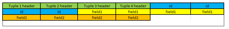
The content of the table would be stored in the following way:

‍

‍

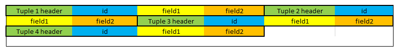
We can see that each tuple has a header followed by the fields (id, field1, and field2). This approach works well for generic data and typical cases. Notice that to add a new tuple, we simply need to put it at the very end of this table (after the last tuple). We can also easily modify the data in place (as long as the data is not getting bigger).

However, this storage type has one big drawback. Computers do not read the data byte by byte. Instead, they bring whole packs of bytes at once and store them in caches. When our application wants to read one byte, the operating system reads 64 bytes or even more like the whole page which is 8kB long. Imagine now that we want to run the following query:

SELECT SUM(field1) FROM test

To execute this query, we need to scan all the tuples and extract one field from each. However, the database engine cannot simply skip other data. It still needs to load nearly whole tuples because it reads a bunch of bytes at once. Let’s see how to make it faster.

‍

What if we stored the data column by column instead? Just like this:

‍

‍

If we now want to extract the field1 column only, we can simply find where it begins and then scan all the values at once. This heavily improves the read performance.

This type of storage is called columnar. We can see that we store each column one after another. In fact, databases store the data independently, so it looks much more like this:

‍

‍

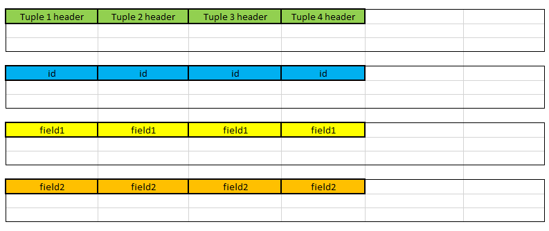
Effectively, the database stores each column separately. Since values within a single column are often similar, we can also compress them or build indexes that can exhibit the similarities, so the scans are even faster.

However, the columnar storage brings some drawbacks as well. For instance, to remove a tuple, we need to delete it from multiple independent storages. Updates are also slower as they may require removing the tuple and adding it back.

One of the solutions that works this way is ParadeDB. It’s an extension to PostgreSQL that uses pg_lakehouse extension to run the queries using DuckDB which is an in-process OLAP database. It’s highly optimized thanks to its columnar storage and can outperform native PostgreSQL by orders of magnitude. They claim they are 94 times faster but it can be even more depending on your use case.

DuckDB is an example of a vectorized query processing engine. It tries to chunk the data into pieces that can fit caches. This way, we can avoid the penalty of expensive I/O operations. Furthermore, we can also use SIMD instructions to perform the same operation on multiple values (thanks to the columnar storage) which improves performance even more.

DuckDB supports two types of indexes:

Min-max (block range) indexes that describe minimum and maximum values in each memory block to make the scans faster. This type of index is also available in native PostgreSQL as BRIN.
Adaptive Radix Tree (ART) indexes to ensure the constraints and speed up the highly selective queries.

While these indexes bring performance benefits, DuckDB cannot update the data. Instead, it deletes the tuples and reinserts them back.

ParadeDB evolved from pg_search and pg_analytics extensions. The latter supports yet another way of storing data if is in parquet format. This format is also based on columnar storage and allows for significant compression.

Automatically Updated Views

Apart from columnar storage, we can optimize how we calculate the data. OLAP workflows often focus on calculating aggregates (like averages) on the data. Whenever we update the source, we need to update the aggregated value. We can either recalculate it from scratch, or we can find a better way to do that.

Hydra boosts the performance of the aggregate queries with the help of pg_ivm. Hydra provides materialized views on the analytical data. The idea is to store the results of the calculated view to not need to recalculate it the next time we query the view. However, if the tables backing the view change, the view becomes out-of-date and needs to be refreshed. pg_ivm introduces the concept of Incremental View Maintenance (IVM) which refreshes the view by recomputing the data using only the subset of the rows that changed.

IVM uses triggers to update the view. Imagine that we want to calculate the average of all the values in a given column. When a new row is added, we don’t need to read all the rows to update the average. Instead, we can use the newly added value and see how it would affect the aggregate. IVM does that by running a trigger when the base table is modified.

Materialized views supporting IVM are called Incrementally Maintainable Materialized Views (IMMV). Hydra provides columnar tables (tables that use columnar storage) and supports IMMV for them. This way, we can get significant performance improvements as data does not need to be recalculated from scratch. Hydra also uses vectorized execution and heavily parallelizes the queries to improve performance. Ultimately, they claim they can be up to 1500 times faster than native PostgreSQL.

Time Series

We already covered many of the workflows that we need to deal with in our day-to-day applications. With the growth of Internet-of-Things (IoT) devices, we face yet another challenge - how to efficiently process billions of signals received from sensors every day.

The data we receive from sensors is called time series. It’s a series of data points indexed in time order. For example, we may be reading the temperature at home every minute or checking the size of the database every second. Once we have the data, we can analyze it and use it for forecasts to detect anomalies or optimize our lives. Time series can be applied to any type of data that is real-valued, continuous, or discrete.

When dealing with time series, we face two problems: we need to aggregate the data efficiently (similarly as in OLAP workflows) and we need to do it fast (as the data changes every second). However, the data is typically append-only and is inherently ordered so we can exploit this time ordering to calculate things faster.

Timescale is an extension for PostgreSQL that supports exactly that. It turns PostgreSQL into a time series database that is efficient in processing any time series data we have. Time series achieves that with clever chunking, IMMV with aggregates, and hypertables. Let’s see how it works.

The main part of Timescale is hypertables. Those are tables that automatically partition the data by time. From the user's perspective, the table is just a regular table with data. However, Timescale partitions the data based on the time part of the entities. The default setting is to partition the data into chunks covering 7 days. This can be changed to suit our needs as we should strive for one chunk consuming around 25% of the memory of the server.

Once the data is partitioned, Timescale can greatly improve the performance of the queries. We don’t need to scan the whole table to find the data because we know which partitions to skip. Timescale also introduces indexes that are created automatically for the hypertables. Thanks to that, we can easily compress the tables and move older data to tiered storage to save money.

The biggest advantage of Timescale is continuous aggregates. Instead of calculating aggregates every time new data is added, we can update the aggregates in real time. Timescale provides three types of aggregates: materialized views (just like regular PostgreSQL’s materialized views), continuous aggregates (just like IMMV we saw before), and real-time aggregates. The last type adds the most recent raw data to the previously aggregated data to provide accurate and up-to-date results.

Unlike other extensions, Timescale supports aggregates on JOINs and can stack one aggregate on top of another. Continuous aggregates also support functions, ordering, filtering, or duplicate removal.

Last but not least, Timescale provides hyperfunctions that are analytical functions dedicated to time series. We can easily bucket the data, calculate various types of aggregates, group them with windows, or even build pipelines for easier processing.

Summary

PostgreSQL is one of the most popular SQL databases. However, it’s not only an SQL engine. Thanks to many extensions, it can now deal with non-relational data, full-text search, analytical workflows, time series, and much more. We don’t need to differentiate between OLAP and OLTP anymore. Instead, we can use PostgreSQL to run HTAP workflows inside one database. This makes PostgreSQL the most versatile database that should easily handle all your needs.

‍