Indexes Under The Hood

Many things can improve database performance. One of the most obvious solutions is to use indexes. This blog post will examine them in detail to understand how they work in PostgreSQL and what makes them useful.

Data Storage Basics

Before getting to indexes, we need to understand the basics of data storage in PostgreSQL. We will explain how things are represented internally, but we won’t cover all the aspects of the data storage like shared memory and buffer pools.

Let’s examine a table. At the very basic level, data is stored in files. There are many files for each table with different content and we’ll examine these types in this article. Let’s begin with the actual data file.

Each file is divided into multiple pages and each page is typically 8 kilobytes long. This makes it easier to manage the growing data without degrading the performance. The database manages pages individually and doesn’t need to load the whole table at once when reading from it. Internally, pages are often called blocks and we will use them interchangeably in this article.

Each data page consists of the following sections:

• Header data - 24 bytes long with some maintenance data for transaction handling and pointers to other sections to find them easily
• Line pointers - pointers to the actual tuples holding the data
• Free space
• Tuples

Let’s see the diagram:

‍

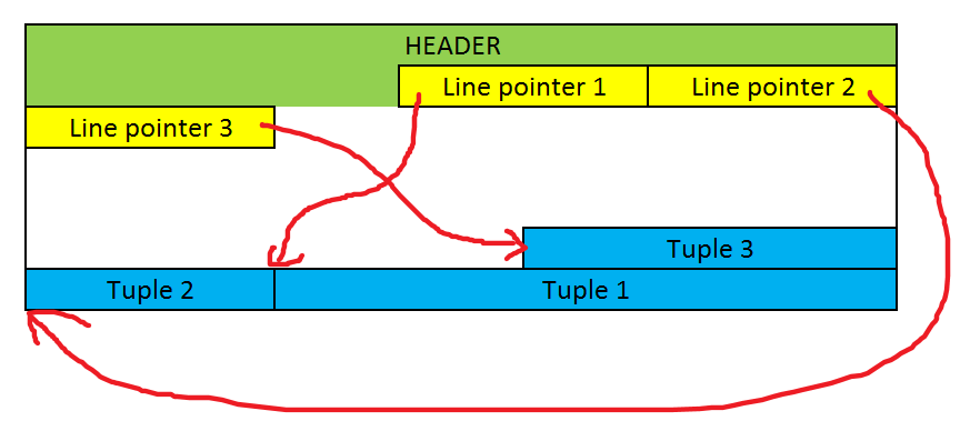
As we can see, tuples are stored backward from the end of the page. Thanks to the pointers, we can easily identify every tuple and we can easily add them to the file.

Each tuple is identified by the Tuple Identifier (TID for short). TID is a pair of numbers indicating the block (page) number and the line pointer number within the page. Effectively, TID indicates the location of the tuple in the physical storage. Once we have the TID, we can easily find the page, then find the pointer, and then jump to the tuple. We don’t need to scan anything along the way as we know where the tuple is.

This is how the tuple looks like typically:

‍

As we can see, each tuple has a header and the actual data. The header stores metadata and some important fields for the transaction handling:

• t_xmin - holds the transaction identifier of the transaction that inserted the tuple
• t_xmax - holds the transaction identifier of the transaction that deleted or updated the tuple. If the tuple hasn’t been deleted or updated yet, 0 is stored here.

Transaction identifier is a number that is incremented with every new transaction. The fields t_xmin and t_xmax are crucial for determining the visibility of the tuple which happens in each transaction. Conceptually, each transaction obtains the transaction snapshot which specifies which tuples should be visible and which should be ignored.

There are many more aspects that we left out in this description like TOAST. We don’t need them to understand the rest of the article but we encourage you to read more about them in our other blog posts.

Internals of Sequential Scan

When reading the table, we would like to achieve the best possible performance. Let’s take the following query:

SELECT * FROM table WHERE id = 123

This query is supposed to extract at most one row. Assuming we have no indexes, the database doesn’t know how many rows meet the filter, so the database needs to scan everything. It needs to go through every tuple one by one and compare it with the filter. This operation is called Sequential Scan. Let’s see how it works.

Conceptually, the operation is very simple. The database just iterates over all files for the table, then iterates over every tuple in the file, compares the tuple using the filter, and then returns only the tuples that meet the criteria. However, since many concurrent operations may be in place, not all tuples should be considered. It is possible that some “future” transactions (transactions that started later than our current transaction) modified the tuples and we shouldn’t include these changes yet as the other transaction hasn’t finished yet (and may need to be rolled back). To decide which tuples we should include, we need to use the transaction snapshot.

Visibility and Transaction Isolation

The rules for obtaining the snapshot depend on the transaction isolation level. For READ COMMITTED, it looks as follows:

‍

1) For each command, the transaction obtains the snapshot
‍
2) When trying to access a tuple, the transaction checks the t_xmin:
‍
3) If the tuple’s t_xmin points to another transaction that is aborted, then the tuple is ignored (as the tuple has been added by some other transaction that was canceled later on and the tuple shouldn’t exist)
‍
4) If the tuple’s t_xmin points to another transaction that is still in progress, then the tuple is ignored (as the tuple has been added by some other transaction that hasn’t completed yet, so the tuple may be removed in the future)
‍


5) If the tuple’s t_xmin points to the current transaction, then it’s visible (as we added this tuple)
‍
6) If the tuple’s t_xmin points to another transaction that is finished, then:
‍
    6a) If the t_xmin is greater than the current transaction identifier, then the tuple is ignored (as it has been added after we started the current transaction so we shouldn’t know about this tuple yet)
‍
    6b) If the t_xmax is 0 or it points to a transaction that was aborted, then the tuple is visible (as the tuple either wasn’t modified or was modified by a transaction that was canceled)
‍
    6c) If the t_xmax points to the current transaction, then the tuple is ignored (as we modified the tuple so there is some new version out there somewhere)
‍
    6d) If the t_xmax points to some other transaction that is still in progress, then the tuple is visible (as someone else is still modifying the tuple but we take the older version)
‍
    6e) If the t_xmax points to another transaction that is committed and is greater than the current transaction, then the tuple is visible (as the tuple has been modified by some transaction from the future, we still take the old version of the tuple)
‍
    6f) Otherwise, the tuple is ignored (as the tuple has been modified by some other transaction that we should respect, to the tuple we’re looking at is now outdated).

As we can see, this protocol is quite complex and has many cases we need to carefully consider. It also depends on the isolation level we use, so there are many more quirks to watch out for.

Cost

We now understand how the sequential scan works. We’re ready to analyze its cost.

Conceptually, every operation consists of two phases. The first phase is the start-up during which we often need to initialize internal structure or precalculate data that we use later on. The second phase is the one in which we extract all tuples and process them accordingly. Therefore, the cost of the operation consists of the start-up cost and run cost.

‍

When it comes to the sequential scan, the start-up cost is zero. The sequential scan doesn’t need to prepare any structures or precalculate any data to process the tuples.

Next, the run cost is the sum of the CPU run cost and disk run cost.

The CPU run cost is the sum of CPU tuple cost and CPU operator cost for each tuple. The former is by default equal to 0.01, and the latter is 0.0025 for this simple comparison. So the CPU run cost is equal to thenumber of tuples multiplied by (0.01 + 0.025) by default.

The disk run cost is equal to the seq page cost multiplied by the number of pages extracted. By default, seq page cost is equal to 1.

As we can see, the total cost of the sequential scan greatly depends on the number of pages read and the number of tuples on each page. Over time, the sequential scan operation will take longer to complete as we add more and more tuples to the table. Even though there is always at most one tuple that meets the criteria (when we search by the identifier), it takes longer to find it as the table grows.

To keep the performance predictable, we need to have a way to find the tuples in constant (or nearly constant) time even if the tables grow. Indexes help us with that. Let’s see how.

Access Methods

PostgreSQL provides a very generic infrastructure for indexes to handle many of them and allow for the open-source development of new ones. Internally, each indexing algorithm is called an access method and is handled in a unified way. We can check what types of indexes we can use with the following query:

SELECT amname FROM pg_am;

‍

As we can see, there are many access methods installed. Each access method provides various options that we can see with the following query:

SELECT a.amname, p.name, pg_indexam_has_property(a.oid,p.name)
FROM pg_am a, UNNEST(ARRAY['can_order','can_unique','can_multi_col','can_exclude', 'can_include']) p(name)
WHERE amname = 'btree';

We can see multiple properties included:

• can_order indicates whether the index supports ASC or DESC during index creation
• can_unique indicates whether this index can enforce the uniqueness constraint
• can_multi_col indicates whether the index can store multiple columns
• can_exclude indicates whether the index supports exclusion constraints when querying
• can_include indicates whether the index supports INCLUDE during creation

We can also query a particular index to check what operations it supports:

select p.name, pg_index_has_property(schema_name.index_name'::regclass, p.name)
from unnest(array[
   	'clusterable','index_scan','bitmap_scan','backward_scan'
 	]) p(name);

These properties indicate the following:

• clusterable - if the index can be used in a CLUSTER command
• index_scan - if the index supports plain (non-bitmap) scans
• bitmap_scan - if the index supports bitmap scans
• backward_scan - if the index scan direction can be changed

As we can see, there are quite a lot of options that we can examine in runtime. What’s more, new access methods can be added dynamically with extensions.

We can also see that one of the access methods is called btree which represents the B-tree type of indexes. This is what we typically mean when we talk about indexes. Let’s see how B-trees work and how they improve the query performance.

B-trees Basics

B-tree is a self-balancing tree data structure that keeps the order of entries. This lets us search entries and insert/delete them in logarithmic time (as compared to linear time with regular heap tables). B-trees generalize the binary search trees and the main difference is that they can have more than two children. They were invented in 1970 and now form the foundation of databases and file systems.

Construction

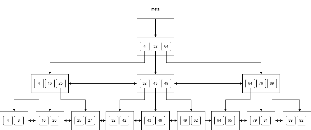
B-trees in PostgreSQL satisfy the following:

• Every node has at most 3 children.
• Every node (except for the root and leaves) has at least 2 children.
• The root node has at least two children (unless the root is a leaf).
• Leaves are on the same level.
• Nodes on the same level have links to siblings.
• Each key in the leaf points to a particular TID.
• Page number 0 of the index holds metadata and points to the tree root.

‍

We can see a sample B-tree below:

‍

When adding a key to a node that is full, we need to split the node into two smaller ones, and then move the key to the parent. This may cause the parent to be split again and the change will propagate up the tree. Similarly, when deleting a key, the tree is kept balanced by merging or redistributing keys among siblings.

Search

When it comes to searching, we can use the binary search algorithm. Let’s say, that we look for a value that appears in the tree only once. This is how we would traverse the tree when looking for 62:

‍

You can see that we just traverse the nodes top-down, check the keys, and finally land at a value. A similar algorithm would work for a value that doesn’t exist in the tree.

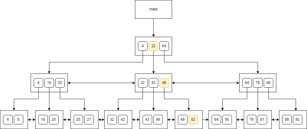
However, we may need to examine multiple values. For instance, when searching for 49:

‍

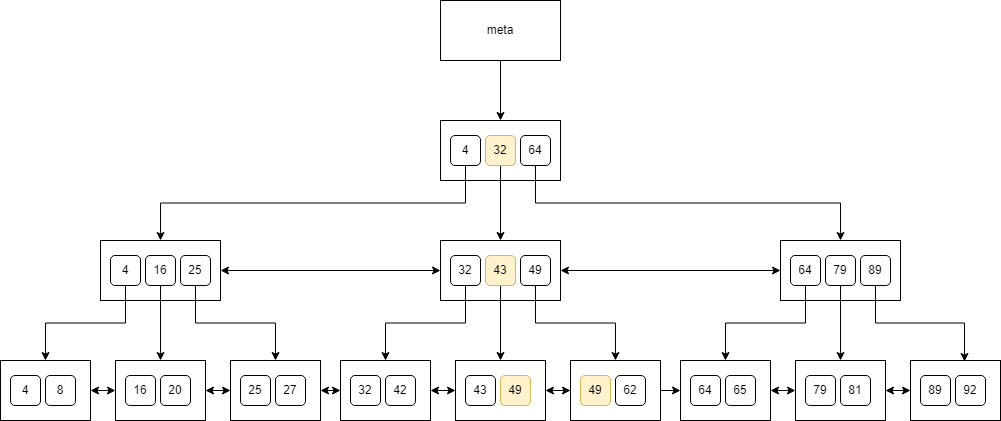
In this case, we first arrive at the leaf, and then we traverse through the siblings to find all the values. We may need to scan multiple nodes in linear time even if we’re looking for equality in the tree. In short, B-trees do not guarantee that we will traverse the tree in the logarithmic time! We may still need to scan the tree linearly.

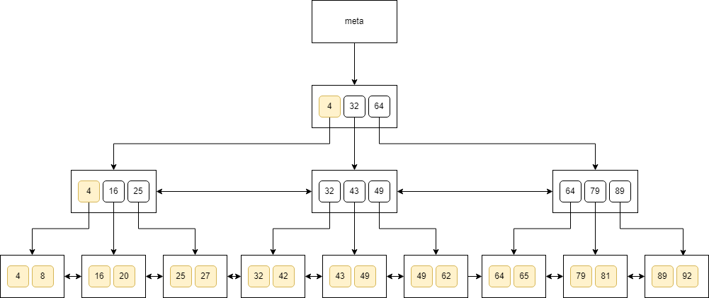
This is more obvious when we look for all the values that are greater than 0:

‍

Multiple Columns

We can also see that B-trees let us traverse the tuples in an ordered manner as the trees maintain the order. We can also traverse them in the reversed order (DESC). The important part here is the order of keys when we include multiple columns.

Let’s say that we created an index with three columns in ascending order:

CREATE INDEX index ON table(column1 ASC, column2 ASC, column3 ASC)

All will work if we query the table with the following order that is aligned with the index construction:

SELECT column1, column2, column3
FROM table
ORDER BY column1, column2, column3

However if we decide to reverse the order of column2, then the query won’t be used:

SELECT column1, column2, column3
FROM table
ORDER BY column1, column2 DESC, column3

To address the issue, we need to create a new index that would sort the columns differently.

Yet another problem occurs if we change the order of columns when sorting:

SELECT column1, column2, column3
FROM table
ORDER BY column1, column3, column2

The index won’t be used because it compares all the columns and we can’t just change the order.

‍

B-trees Internals

Let’s now see some internals of B-trees and how they can affect the performance.

CREATE INDEX index ON table(column1)

SELECT column1, column2
FROM table

We can’t extract column2 from the index itself. We need to access the table which makes it much slower. However, to make the index not go to the table to fetch the column, we can include additional columns. This is called a covering index:

CREATE INDEX index ON table(column1) INCLUDE(column2)

Once we create a covering index, the engine doesn’t need to fetch the column from the table and can use index only.

Visibility Maps

One thing that we ignored in the discussion is how to verify the visibility of the tuples. Notice that the index doesn’t have the t_xmin and t_xmax. To use the tuple, we need to verify if the current transaction should see it or not. When we discussed the sequential scan, we explained that this is done for each tuple based on the transaction isolation level. The same must be done when using the index.

Unfortunately, there is no magical solution here. When scanning the index, we need to access each tuple in the table and check the t_xmin and t_xmax according to the transaction snapshot that we discussed below. However, we can precalculate some data. This is called a visibility map.

The visibility map is a bitset that answers if all the tuples in a given page are visible to all transactions. We can maintain such a bitmap and use it when scanning the index. When we find the key in the index that meets the criteria, we can consult the visibility map and check if the tuple is visible to all the transactions. If that’s the case, then we don’t need to access the table at all (assuming the index is a covering index). If the visibility map claims otherwise, then we need to check the tuple in the table using the regular logic.

The visibility map is updated during transactions (when we modify tuples) and during VACUUMING. 

Comparison Operators

The B-tree index needs to know how to order values. It’s rather straightforward for built-in types but may require some additions when dealing with custom types.

It’s important to understand that data types may not have any ordering. For instance, there is no “natural” ordering for two-dimensional points on a plane. You may sort them based on their X value or you may go with distance from the point (0,0). Since there are many orderings possible, you need to define which one you’d like to use. PostgreSQL lets you do that with operator families.

Each operator family defines operators that we can use. Each operator is assigned to a strategy (less, less or equal, equal, greater or equal, greater) that explains what the operator does. We can check which operators are used by the B-tree for “less than” operation with the following query:

SELECT amop.amopopr::regoperator as opfamily_operator
FROM pg_am am, pg_opfamily opf, pg_amop amop
WHERE opf.opfmethod = am.oid AND amop.amopfamily = opf.oid AND am.amname = 'btree' AND opf.opfname = 'integer_ops' AND amop.amopstrategy = 1
ORDER BY opfamily_operator;

This explains what operators are used for what data types. If you want to support the B-tree index for your custom type, you need to create an operator class and register it for the B-tree like this:

CREATE OPERATOR CLASS operator_class
DEFAULT FOR TYPE your_type
USING btree AS
	OPERATOR 1 less_operator,
	OPERATOR 2 less_or_equal_operator,
	OPERATOR 3 equal_operator,
	OPERATOR 4 greater_or_equal_operator,
	OPERATOR 5 greater_operator,
	FUNCTION 1 your_type_comparator(your_type, your_type);

Index Scan Cost

Just like with the sequential scan, the index scan function needs to estimate the cost properly.

The start-up cost depends on the number of tuples in the index and the height of the index. It is specified as cpu_operator_cost multiplied by the ceiling of the base-2 logarithm of the number of tuples plus the height of the tree multiplied by 50.

The run cost is the sum of the CPU cost (for both the table and the index) and the I/O cost (again, for the table and the index).

The CPU cost for the index is calculated as the sum of constants cpu_index_tuple_cost and qual_op_cost (which are 0.005 and 0.0025 respectively) multiplied by the number of tuples in the index multiplied by the selectivity of the index.

Selectivity of the index is the estimate of how many values inside the index would match the filtering criteria. It is calculated based on the histogram that captures the counts of the values. The idea is to divide the column’s values into groups of approximately equal populations to build the histogram. Once we have such a histogram, we can easily specify how many values should match the filter.

The CPU cost for the table is calculated as the cpu_tuple_cost (constant 0.01) multiplied by the number of tuples in the table multiplied by the selectivity. Notice that this assumes that we’ll need to access each tuple from the table even if the index is covering.

The I/O cost for the index is calculated as the number of pages in the index multiplied by the selectivity multiplied by the random_page_cost which is set to 4.0 by default.

Finally, the I/O cost for the table is calculated as the sum of the number of pages multiplied by the random_page_cost and the index correlation multiplied by the difference between the worst-case I/O cost and the best-case I/O cost. The correlation indicates how much the order of tuples in the index is aligned with the order of tuples in the table. It can be between -1.0 and 1.0.

All these calculations show that index operations can be beneficial if we extract only a subset of rows. It’s no surprise that the index scans will be even more expensive than the sequential scans, but the index seeks will be much faster.

Internals Inspection

We can use the pageinspect extension to analyze the index easily:

CREATE EXTENSION pageinspect;

For instance, this is how we can read the index metapage:

SELECT * FROM bt_metap('schema_name.index_name');

This shows how many levels the index has. We can also check the page of the index:

SELECT * FROM bt_page_stats('schema_name.index_name', 1);

This shows the number of tuples on this particular page. We can even check the data in the block to see the index’s content:

SELECT itemoffset, ctid, itemlen, LEFT(data,56) AS data
FROM bt_page_items('imdb.title_ratings_idx', 1) limit 5;

You can easily see where the rows are stored. Consult the documentation to read more about the internals.

Summary

B-tree indexes are the most popular ones. They can greatly improve the performance of reads and seeks and can avoid accessing the tables entirely. In this blog post, we examined how PostgreSQL stores the data, how it performs a sequential scan, and how B-tree indexes help with fetching the data. We also covered the transaction isolation levels and how PostgreSQL calculates the visibility of the tuples. Many more indexes in PostgreSQL use different approaches and it’s always beneficial to examine their internals to achieve the best possible performance.

‍